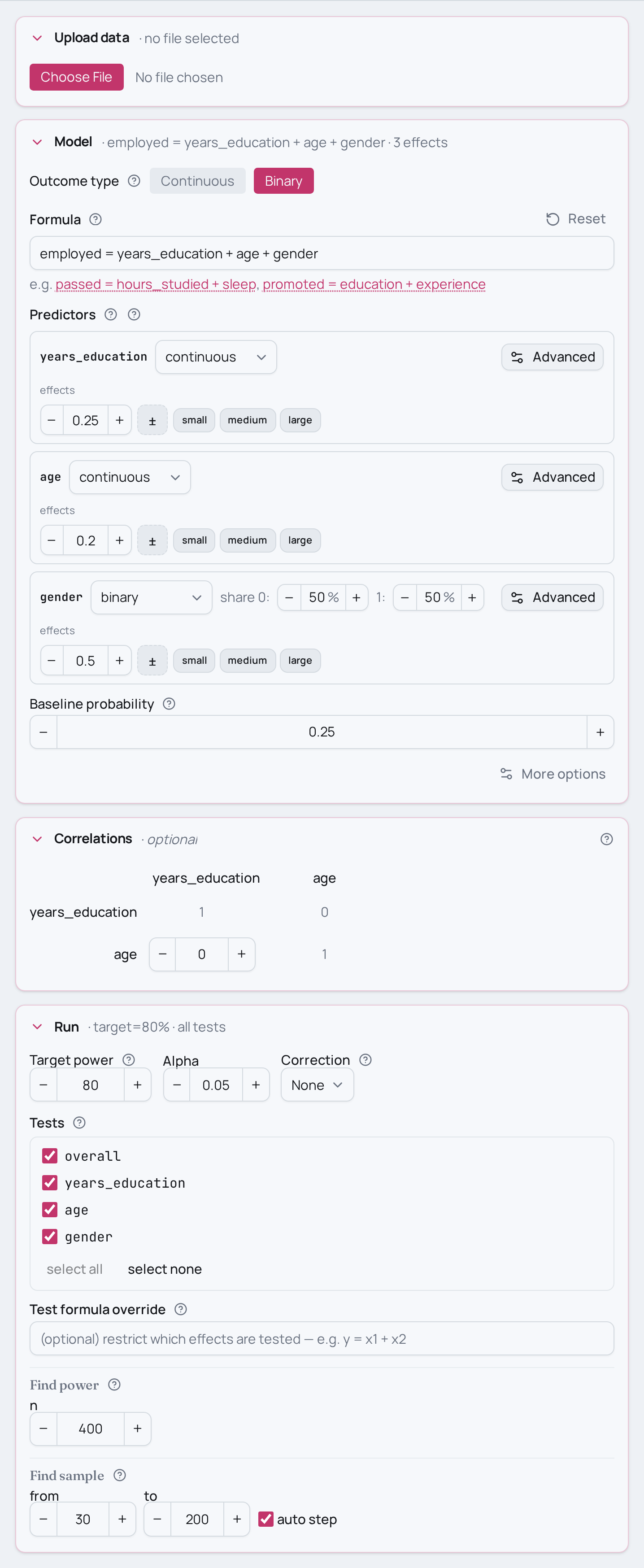
Power for multiple logistic regression (adjusted)

Your outcome is binary — a respondent is employed or not — and you have a single predictor whose effect you actually care about, years_education, plus covariates (age, gender) you carry along only to control for confounding. The question is the power to detect the adjusted education effect: the partial log-odds coefficient once the covariates have soaked up their share of the employment difference.

As an MCPower formula: employed ~ years_education + age + gender, estimated by the GLM (logit-link) estimator via family="logit", with target_test = "years_education" so the headline power is for the key predictor alone. gender is a binary 0/1 covariate; age and years_education are continuous. The covariates correlate with the predictor — that overlap is the whole reason you adjust, and it is what drives the partial coefficient's power down relative to an unadjusted look. A logit model also needs a baseline event rate, set with set_baseline_probability, which fixes the intercept.

Variations

A rarer or commoner outcome. Change set_baseline_probability(0.25) — a rarer employment base rate (say 0.10) carries less information per observation and lowers power for every coefficient at a fixed N.
Different confounding strength. Raise or lower the corr(years_education, …) terms: stronger covariate–predictor correlation steals more variance from the partial coefficient and lowers power for years_education.
More or fewer controls. Drop gender, or add a third covariate — each extra control costs a degree of freedom and shifts the adjusted power.
A 3-level covariate. Swap the binary gender for a categorical control with set_variable_type("region=(factor,3)") and a 0.20/0.50/0.80 effect-size benchmark per category.
Solve for N instead. Swap find_power(sample_size=400, …) for find_sample_size(target_test="years_education", from_size=…, to_size=…, by=…) to get the N that lands the education effect at 80% power.
Same design, other fields:
- relapse ~ biomarker_level + age + dose — does biomarker level predict relapse after adjusting for age and dose? (clinical)
- germinated ~ soil_nitrogen + moisture + temperature — does soil nitrogen predict germination after controlling for moisture and temperature? (ecology)

Not this setup?

If you'd rather have…

Regression with many continuous controls (adjusted association) — Same covariate-adjusted multi-predictor association, but for a continuous outcome (OLS) instead of a binary one.
Mixed binary + continuous predictors (parallel slopes) — The linear-outcome analogue of the same mixed binary + continuous predictor set with parallel slopes.
Logistic continuous-by-continuous moderation — Stay logistic but test an interaction (moderation) between predictors rather than covariate adjustment.
Logistic treatment-by-moderator interaction (binary x continuous) — Logistic with a treatment-by-moderator interaction if you want an effect that varies by a covariate instead of plain adjustment.

Copy-paste setup

from mcpower import MCPower

# Covariate-adjusted logistic association: does `years_education` predict whether a
# person is employed (yes/no), holding age and gender constant?
# family="logit" makes the outcome binary — the engine fits a GLM (logit link)
# on every Monte Carlo iteration.
model = MCPower("employed = years_education + age + gender", family="logit")

# years_education and age are continuous (default); gender is a binary 0/1 predictor.
model.set_variable_type("gender=binary")

# Baseline probability — the employment rate when every predictor is at its
# reference value. Required for logit; it sets the model intercept via
# log(p / (1 - p)). Here 25% of reference individuals are employed.
model.set_baseline_probability(0.25)

# Standardised effects (log-odds shifts).
#   years_education=0.25 -> the key predictor, a medium adjusted association (continuous benchmark).
#   age=0.20             -> a continuous nuisance covariate carried along for adjustment.
#   gender=0.50          -> a binary covariate, medium on the binary benchmark scale.
model.set_effects("years_education=0.25, age=0.20, gender=0.50")

# Age correlates with years of education — that confounding is the reason we adjust,
# and it changes the power for the years_education coefficient. Correlations are only
# defined between continuous variables, so gender (binary) cannot be correlated
# here; it enters from its own marginal.
model.set_correlations("corr(years_education, age)=0.3")

model.find_power(sample_size=400, target_test="years_education")

suppressMessages(library(mcpower))

# Covariate-adjusted logistic association: does `years_education` predict whether a
# person is employed (yes/no), holding age and gender constant?
# family="logit" makes the outcome binary — the engine fits a GLM (logit link)
# on every Monte Carlo iteration.
model <- MCPower$new("employed ~ years_education + age + gender", family = "logit")

# years_education and age are continuous (default); gender is a binary 0/1 predictor.
model$set_variable_type("gender=binary")

# Baseline probability — the employment rate when every predictor is at its
# reference value. Required for logit; it sets the model intercept via
# log(p / (1 - p)). Here 25% of reference individuals are employed.
model$set_baseline_probability(0.25)

# Standardised effects (log-odds shifts).
#   years_education=0.25 -> the key predictor, a medium adjusted association (continuous benchmark).
#   age=0.20             -> a continuous nuisance covariate carried along for adjustment.
#   gender=0.50          -> a binary covariate, medium on the binary benchmark scale.
model$set_effects("years_education=0.25, age=0.20, gender=0.50")

# Age correlates with years of education — that confounding is the reason we adjust,
# and it changes the power for the years_education coefficient. Correlations are only
# defined between continuous variables, so gender (binary) cannot be correlated
# here; it enters from its own marginal.
model$set_correlations("corr(years_education, age)=0.3")

model$find_power(sample_size = 400, target_test = "years_education")