Power for logistic regression with a categorical control

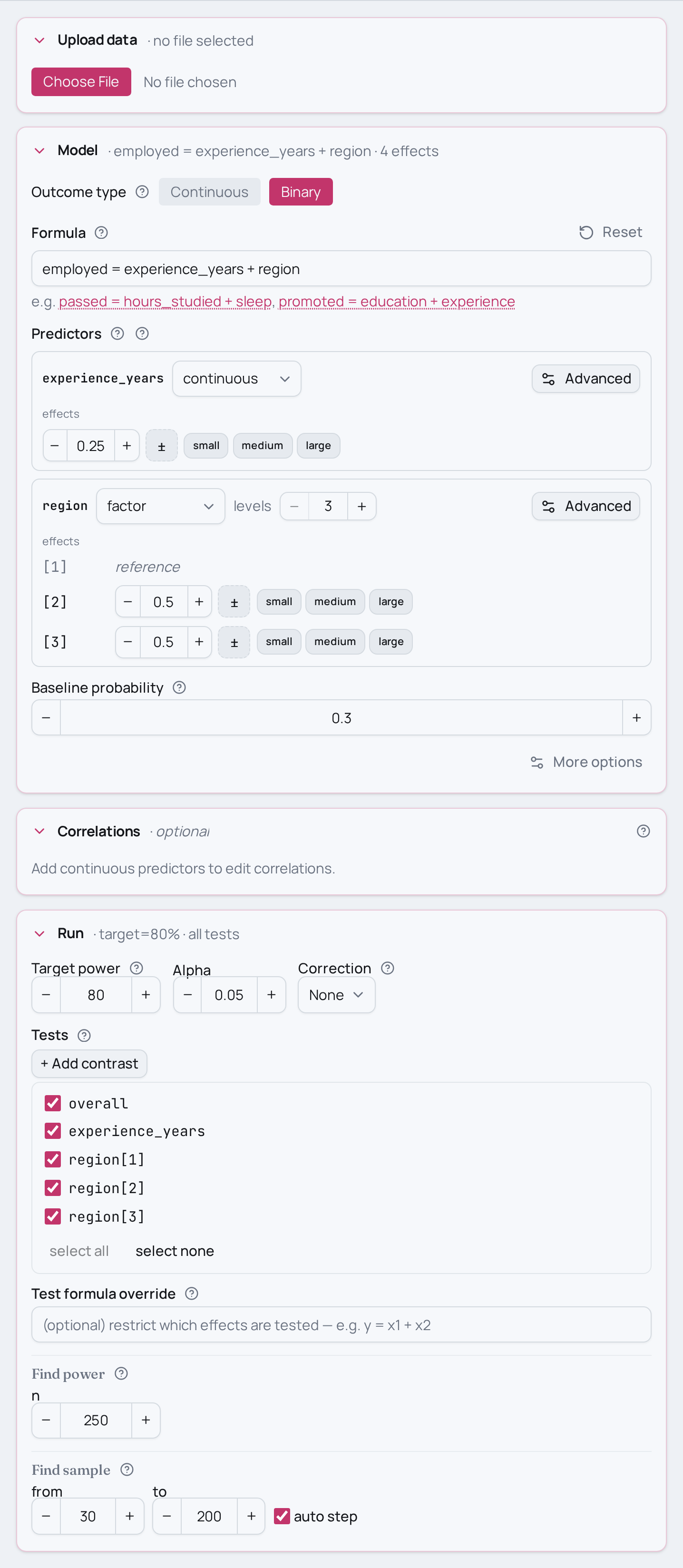
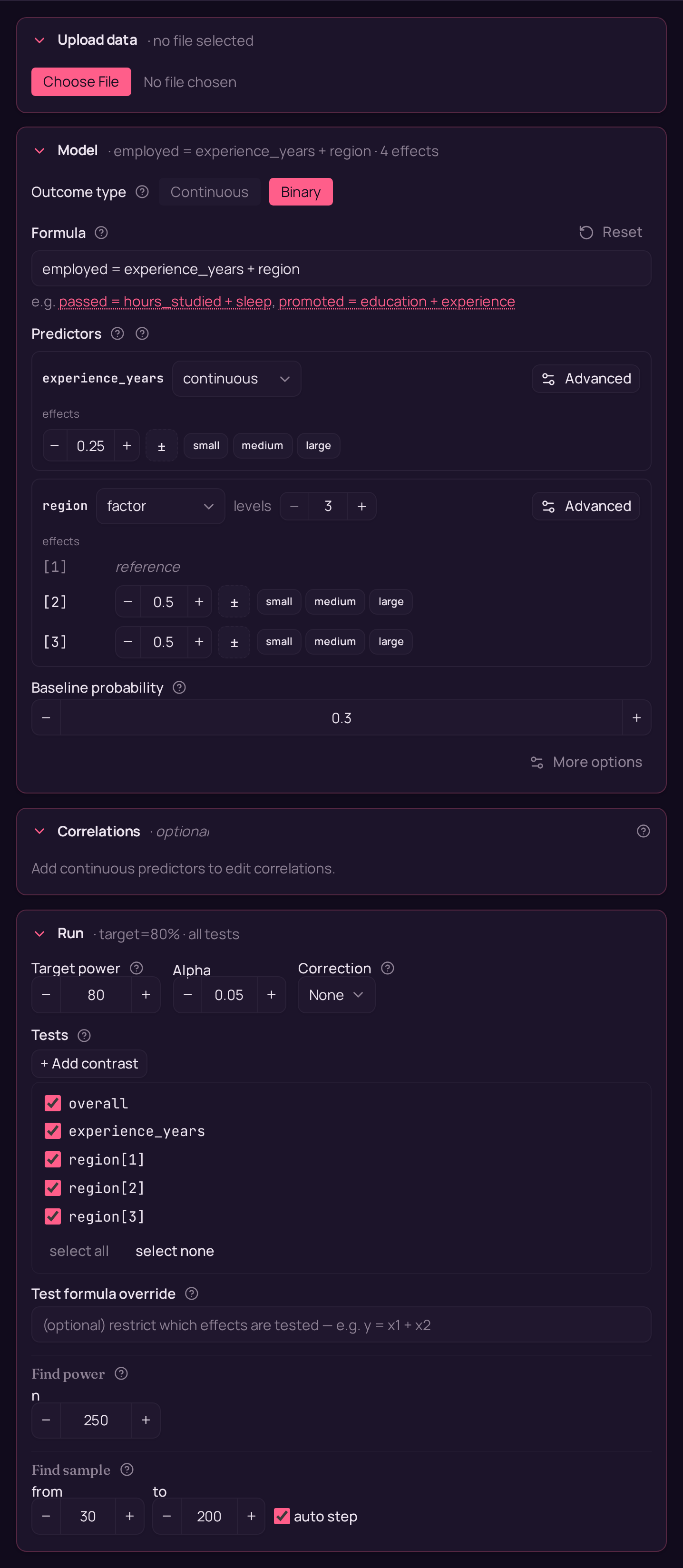
A yes/no outcome driven by one continuous predictor, but the comparison only makes sense after you hold a grouping variable constant. Does a respondent's experience_years shift the odds of being employed once you account for which region they live in — keeping the experience slope parallel across regions? As an MCPower formula this is employed ~ experience_years + region with family="logit": a binary outcome, one continuous predictor of interest, and a multi-level categorical control entered additively (no interaction — same slope in every region).

Variations

• Dial the expected association up or down by changing the continuous effect: experience_years=0.10 for a small relationship, experience_years=0.40 for a large one (the medium benchmark for a continuous predictor is 0.25).
• Change how many regions you control for by editing the factor level count: region=(factor,4) for four regions instead of three (the factor effect stays on the 0.20 / 0.50 / 0.80 benchmark scale).
• Swap the categorical control for a binary one — region=binary makes it a two-group control, the simplest covariate-adjusted logistic model.
• Searching for the sample size that reaches 80% power instead of scoring a fixed N? Swap find_power(sample_size=250, ...) for find_sample_size(target_test="experience_years", from_size=100, to_size=600, by=20).
• Same design, other fields:
  • relapse ~ biomarker_level + clinic — does biomarker level predict relapse after controlling for clinic site? (clinical)
  • germinated ~ soil_nitrogen + habitat — does soil nitrogen predict germination after accounting for habitat type? (ecology)

Not this setup?

• Adjusted binary-outcome model with covariates
• Multi-level categorical predictor (survived ~ habitat)
• Simple logistic regression with one continuous predictor

If you'd rather have…

• Moderation between two predictors — make the two predictors interact (continuous-by-continuous moderation) instead of adjusting additively.
• Binary-by-continuous interaction — let the categorical control moderate the continuous effect (binary-by-continuous interaction) rather than parallel slopes.
• Covariate-adjusted continuous outcome (ANCOVA) — the same continuous-plus-control structure but for a continuous outcome instead of a binary one.
• Two-group proportion comparison — drop the continuous predictor for a plain two-group logistic comparison.

Copy-paste setup

from mcpower import MCPower

# Covariate-adjusted logistic regression (parallel slopes on the log-odds).
# Research question: does years of work experience shift the probability of
# employment once we account for which region the respondent lives in?
# family="logit" makes employed a binary (0/1) outcome fitted by a logistic GLM.
model = MCPower("employed = experience_years + region", family="logit")

# region is a categorical control with 3 levels -> 2 dummy contrasts.
model.set_variable_type("region=(factor,3)")

# Expected effects on the standardised benchmark scales.
#   experience_years=0.25   -> a medium continuous association with the log-odds.
#   region[2]/[3]           -> a medium factor effect for each non-reference region
#                              (effects are set per dummy contrast, not on the bare factor).
model.set_effects("experience_years=0.25, region[2]=0.50, region[3]=0.50")

# Logistic GLMs need a baseline event rate to anchor the intercept: at the
# reference region and average experience, 30% of respondents are employed.
model.set_baseline_probability(0.30)

# Power at N=250, targeting the adjusted experience effect (region held constant).
model.find_power(sample_size=250, target_test="experience_years")

suppressMessages(library(mcpower))

# Covariate-adjusted logistic regression (parallel slopes on the log-odds).
# Research question: does years of work experience shift the probability of
# employment once we account for which region the respondent lives in?
# family = "logit" makes employed a binary (0/1) outcome fitted by a logistic GLM.
model <- MCPower$new("employed ~ experience_years + region", family = "logit")

# region is a categorical control with 3 levels -> 2 dummy contrasts.
model$set_variable_type("region=(factor,3)")

# Expected effects on the standardised benchmark scales.
#   experience_years=0.25   -> a medium continuous association with the log-odds.
#   region[2]/[3]           -> a medium factor effect for each non-reference region
#                              (effects are set per dummy contrast, not on the bare factor).
model$set_effects("experience_years=0.25, region[2]=0.50, region[3]=0.50")

# Logistic GLMs need a baseline event rate to anchor the intercept: at the
# reference region and average experience, 30% of respondents are employed.
model$set_baseline_probability(0.30)

# Power at N=250, targeting the adjusted experience effect (region held constant).
invisible(model$find_power(sample_size = 250, target_test = "experience_years"))