Power analysis for a logistic two-group comparison

You have a yes/no outcome — remission vs no remission — and two groups (control vs active treatment), and you want to know whether the remission rate differs between them. This is the two-group logistic comparison, written here as a regression on a single binary predictor: remission ~ treatment.

Variations

Smaller or larger gap. The effect is on the binary benchmark scale — swap treatment=0.50 (medium) for treatment=0.20 (small) or treatment=0.80 (large) to see how the expected separation between the two remission rates moves power.
Different control remission rate. The baseline probability anchors how common remission is in the control group — move set_baseline_probability(0.20) to a rarer (0.05) or more common (0.50) base rate; rare events cost power for the same total N.
Unbalanced groups. If you expect a lopsided split rather than 50/50, set the treatment proportion when you declare the variable type — unbalanced cells cost power for the same total N.
Solve for N instead. Replace find_power(sample_size=200, …) with find_sample_size(target_test="treatment", from_size=50, to_size=500, by=25) to get the minimum N that reaches 80% power.
Same design, other fields:
- survived ~ predator_present — does predator presence shift seedling survival rates? (ecology)
- voted ~ union_member — do union members turn out to vote at different rates than non-members? (social science)

Not this setup?

If you'd rather have…

A 3+-level treatment instead of two groups — same two-group logistic comparison but with 3+ treatment levels instead of two: the multi-level categorical extension of this binary-predictor design.
A measured predictor instead of a two-group split — logistic regression with a single continuous predictor instead of a binary group; switch when your predictor is measured, not a two-group split.
The covariate-adjusted version of this comparison — keeps the binary group effect but adjusts for covariates (age, gender): the covariate-adjusted version of this two-group comparison.
The same two groups on a continuous outcome — the exact same two-group design on a continuous outcome (independent t-test as regression); use when the outcome is numeric rather than a binary event.
The clustered (cluster-randomized) version — two-group binary outcome but with clustering (random intercept per cluster): the mixed-model version for cluster-randomized binary trials.

Copy-paste setup

from mcpower import MCPower

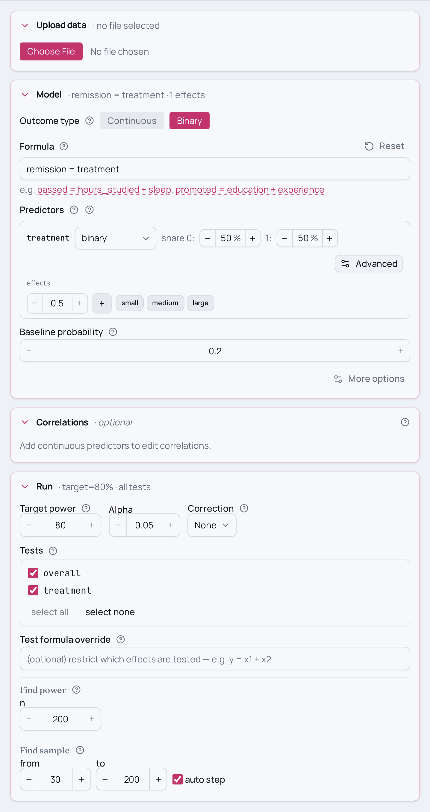
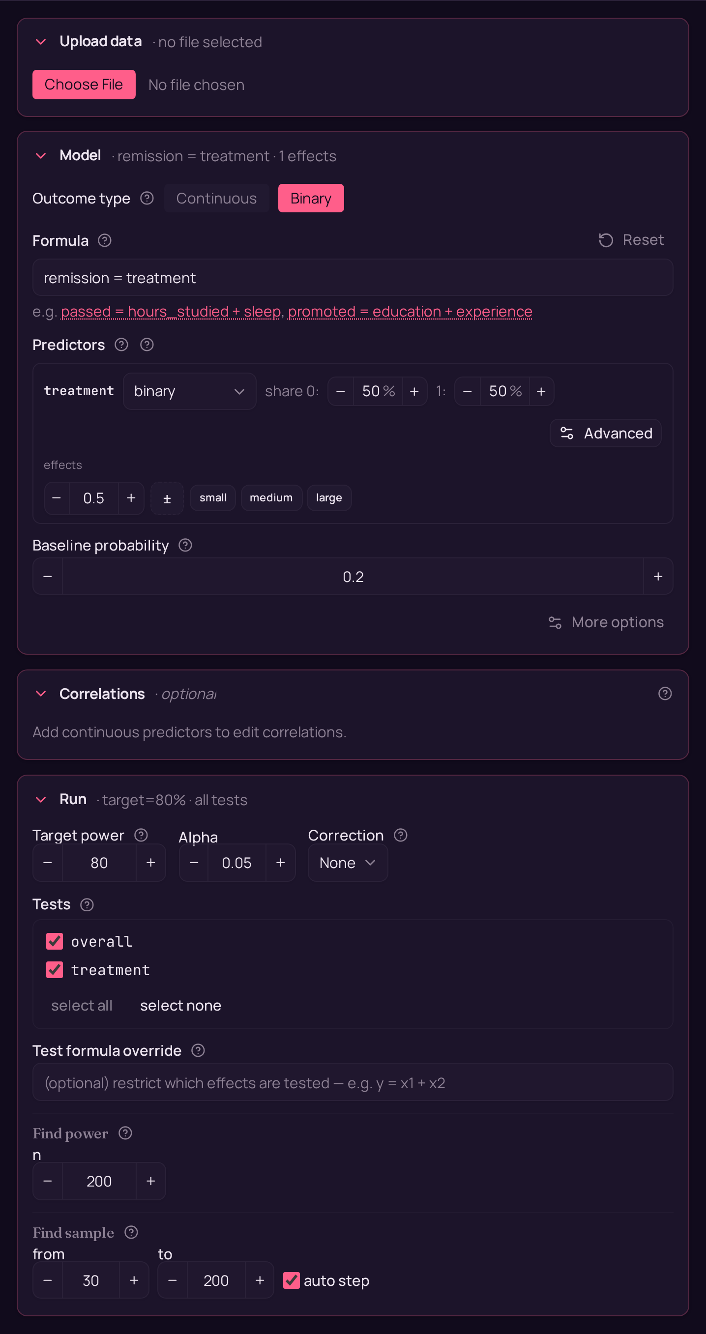
# Two-group comparison on a binary (remission / no-remission) outcome: logistic regression.
model = MCPower("remission = treatment", family="logit")

# treatment is a binary two-level predictor (0 = control, 1 = active treatment).
model.set_variable_type("treatment=binary")

# Expected group effect on the binary benchmark scale: 0.50 = a medium gap.
model.set_effects("treatment=0.50")

# Remission rate in the control group (logit family needs a baseline probability).
model.set_baseline_probability(0.20)

model.find_power(sample_size=200, target_test="treatment")

suppressMessages(library(mcpower))

# Two-group comparison on a binary (remission / no-remission) outcome: logistic regression.
model <- MCPower$new("remission ~ treatment", family = "logit")

# treatment is a binary two-level predictor (0 = control, 1 = active treatment).
model$set_variable_type("treatment=binary")

# Expected group effect on the binary benchmark scale: 0.50 = a medium gap.
model$set_effects("treatment=0.50")

# Remission rate in the control group (logit family needs a baseline probability).
model$set_baseline_probability(0.20)

invisible(model$find_power(sample_size = 200, target_test = "treatment"))