Power analysis for ANCOVA (covariate-adjusted)

You have two groups — a treatment arm and a control arm — and a continuous baseline blood pressure measurement taken before the intervention. Comparing the groups on raw blood pressure wastes the baseline information; adjusting for it soaks up between-patient variability and sharpens the treatment estimate. This is the classic ANCOVA: a binary treatment effect read off net of a continuous covariate, with the two groups sharing one common slope on baseline_bp (parallel slopes).

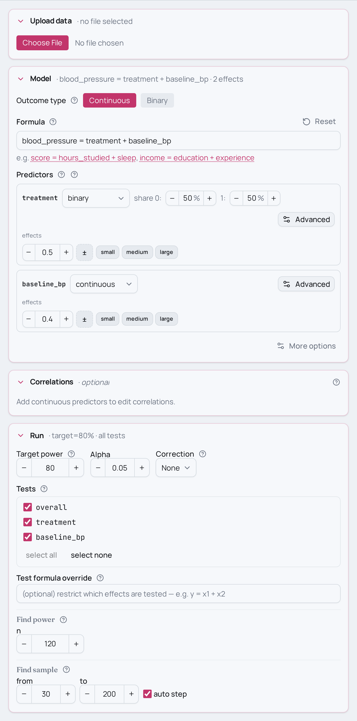
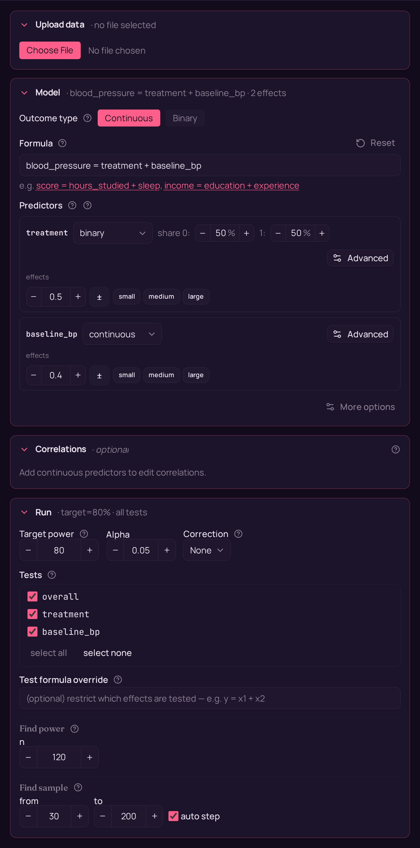
The model is blood_pressure ~ treatment + baseline_bp — the adjusted treatment effect plus a continuous control, fit by OLS.

Variations

• Suspect the treatment works differently across the baseline range? Let the slopes diverge by adding a treatment:baseline_bp interaction — that turns the parallel-slopes assumption into something you actually test rather than assume.
• More than two arms. Swap the binary treatment for a 3-level factor dose_level (e.g. dose_level[2], dose_level[3]); the page stays an ANCOVA, now with a multi-level adjusted comparison.
• Several covariates. Add more continuous controls — blood_pressure ~ treatment + baseline_bp + age — when one pre-treatment measurement isn't the only thing that drives the outcome.
• A weaker covariate. Dial baseline_bp down to the 0.25 medium benchmark (or 0.10 small) when the baseline only loosely predicts the outcome — the adjustment buys you less, so the treatment effect needs more N to clear power.
• Same design, other fields:
  • Ecology: plant_biomass ~ habitat + soil_nitrogen — does habitat type shift plant biomass adjusting for baseline soil nitrogen?
  • Social science: wage ~ gender + experience_years — does a gender gap in wages persist after adjusting for years of experience?

Not this setup?

• Same group + baseline design with a group-by-baseline interaction — when you want to test whether the treatment effect depends on the covariate.
• Two-group comparison with no covariate — the independent t-test as regression, without baseline adjustment.
• The same parallel-slopes model framed as sex + age rather than treatment + baseline.

If you'd rather have…

• A test of homogeneity of slopes — same group + baseline design but adds a group-by-baseline interaction to check whether the treatment effect depends on the covariate.
• The unadjusted two-group test — drop the covariate entirely and just compare the two groups (independent t-test as regression).
• The same structure with different names — a binary + continuous parallel-slopes model framed as sex + age.
• The ANOVA-family analog — covariate-adjusted factorial design (two-way ANCOVA) when you want omnibus F-tests instead of regression coefficients.
• Several continuous covariates at once — isolate one predictor's association net of multiple controls instead of a single baseline.

Copy-paste setup

from mcpower import MCPower

# Covariate-adjusted two-group comparison (ANCOVA-style, parallel slopes).
# Research question: does the treatment shift blood_pressure once we adjust for
# each patient's baseline_bp measurement?
model = MCPower("blood_pressure = treatment + baseline_bp")

# Expected effect sizes (standardised).
#   treatment=0.50   → treatment shifts blood_pressure by a medium binary effect.
#   baseline_bp=0.40 → baseline_bp is a strong continuous covariate.
model.set_effects("treatment=0.50, baseline_bp=0.40")

# Variable types — treatment is binary (0=control, 1=treatment); baseline_bp stays
# continuous by default.
model.set_variable_type("treatment=binary")

# Power at N=120, targeting the adjusted treatment effect.
model.find_power(sample_size=120, target_test="treatment")

suppressMessages(library(mcpower))

# Covariate-adjusted two-group comparison (ANCOVA-style, parallel slopes).
# Research question: does the treatment shift blood_pressure once we adjust for
# each patient's baseline_bp measurement?
model <- MCPower$new("blood_pressure ~ treatment + baseline_bp")

# Expected effect sizes (standardised).
#   treatment=0.50   -> treatment shifts blood_pressure by a medium binary effect.
#   baseline_bp=0.40 -> baseline_bp is a strong continuous covariate.
model$set_effects("treatment=0.50, baseline_bp=0.40")

# Variable types — treatment is binary (0=control, 1=treatment); baseline_bp stays
# continuous by default.
model$set_variable_type("treatment=binary")

# Power at N=120, targeting the adjusted treatment effect.
invisible(model$find_power(sample_size = 120, target_test = "treatment"))