Power for a covariate-adjusted OLS effect

You have a single predictor whose effect you actually care about — years_education — and a set of continuous covariates (age, experience_years, tenure) you carry along only to control for confounding. The question is the power to detect the adjusted years_education effect, the partial coefficient once the covariates have soaked up their share of the outcome.

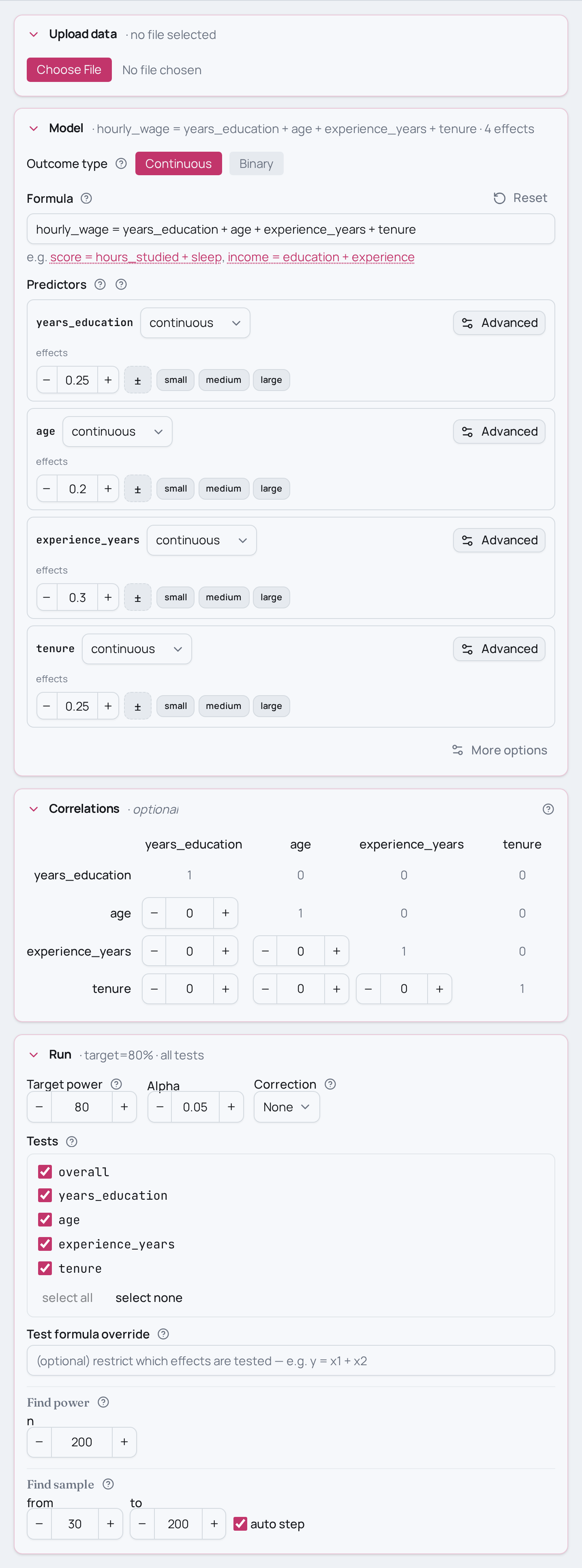
As an MCPower formula: hourly_wage ~ years_education + age + experience_years + tenure, estimated by OLS, with target_test = "years_education" so the headline power is for the key predictor alone. The covariates are correlated with years_education — that overlap is the whole reason you adjust, and it is what drives the partial coefficient's power down relative to an unadjusted look.

Variations

• Different confounding strength. Raise or lower the corr(years_education, …) terms: stronger covariate–predictor correlation steals more variance from the partial coefficient and lowers power for years_education at a fixed N.
• More or fewer controls. Drop tenure, or add a fourth covariate — each extra control costs a degree of freedom and shifts the adjusted power.
• Solve for N instead. Swap find_power(sample_size=200, …) for find_sample_size(target_test="years_education", from_size=…, to_size=…, by=…) to get the N that lands the years_education effect at 80% power.
• A categorical predictor of interest. Replace the continuous years_education with a binary group (set_variable_type("years_education=binary")) and a 0.20/0.50/0.80 effect-size benchmark to model a treatment-vs-control contrast under adjustment.
• Same design, other fields:
  • Clinical: cholesterol ~ dose + age + baseline_bp + biomarker_level — adjusted effect of dose on cholesterol holding several clinical covariates constant.
  • Ecology: plant_biomass ~ rainfall + soil_nitrogen + temperature + moisture — adjusted effect of rainfall on biomass controlling for several environmental covariates.

Not this setup?

• Multiple regression, three continuous predictors
• Mixed binary + continuous predictors (parallel slopes)
• ANCOVA: group effect adjusting for a baseline covariate
• Multiple logistic regression: covariate-adjusted binary outcome

If you'd rather have…

• Multiple regression, three continuous predictors — Fewer controls: a plain three-continuous-predictor multiple regression without the single-predictor-of-interest framing.
• Two-predictor multiple regression — The minimal adjusted model: one predictor plus a single covariate.
• ANCOVA: group effect adjusting for a baseline covariate — If your key predictor is a group/treatment and you only need to adjust for one baseline covariate (ANCOVA).
• Multiple logistic regression: covariate-adjusted binary outcome — Same covariate-adjusted association but with a binary outcome (multiple logistic regression).
• Continuous moderation with a covariate — If you also want the predictor of interest to interact with a moderator while still adjusting for a covariate.

Copy-paste setup

from mcpower import MCPower

# Covariate-adjusted association: the effect of `years_education` on `hourly_wage`,
# holding age, experience_years, and tenure constant. All four predictors are continuous.
model = MCPower("hourly_wage = years_education + age + experience_years + tenure")

# Standardised effect sizes (continuous benchmark scale).
#   years_education=0.25  -> the key predictor, a medium adjusted association.
#   age/experience_years/tenure -> nuisance covariates carried along for adjustment.
model.set_effects("years_education=0.25, age=0.20, experience_years=0.30, tenure=0.25")

# Covariates correlate with years_education — that confounding is the reason we
# adjust, and it changes the power for the years_education coefficient.
model.set_correlations(
    "corr(years_education, age)=0.3, "
    "corr(years_education, experience_years)=0.4, "
    "corr(experience_years, tenure)=0.5"
)

model.find_power(sample_size=200, target_test="years_education")

suppressMessages(library(mcpower))

# Covariate-adjusted association: the effect of `years_education` on `hourly_wage`,
# holding age, experience_years, and tenure constant. All four predictors are continuous.
model <- MCPower$new("hourly_wage ~ years_education + age + experience_years + tenure")

# Standardised effect sizes (continuous benchmark scale).
#   years_education=0.25  -> the key predictor, a medium adjusted association.
#   age/experience_years/tenure -> nuisance covariates carried along for adjustment.
model$set_effects("years_education=0.25, age=0.20, experience_years=0.30, tenure=0.25")

# Covariates correlate with years_education — that confounding is the reason we
# adjust, and it changes the power for the years_education coefficient.
model$set_correlations(paste0(
  "corr(years_education, age)=0.3, ",
  "corr(years_education, experience_years)=0.4, ",
  "corr(experience_years, tenure)=0.5"
))

model$find_power(sample_size = 200, target_test = "years_education")