Power for OLS with three continuous predictors

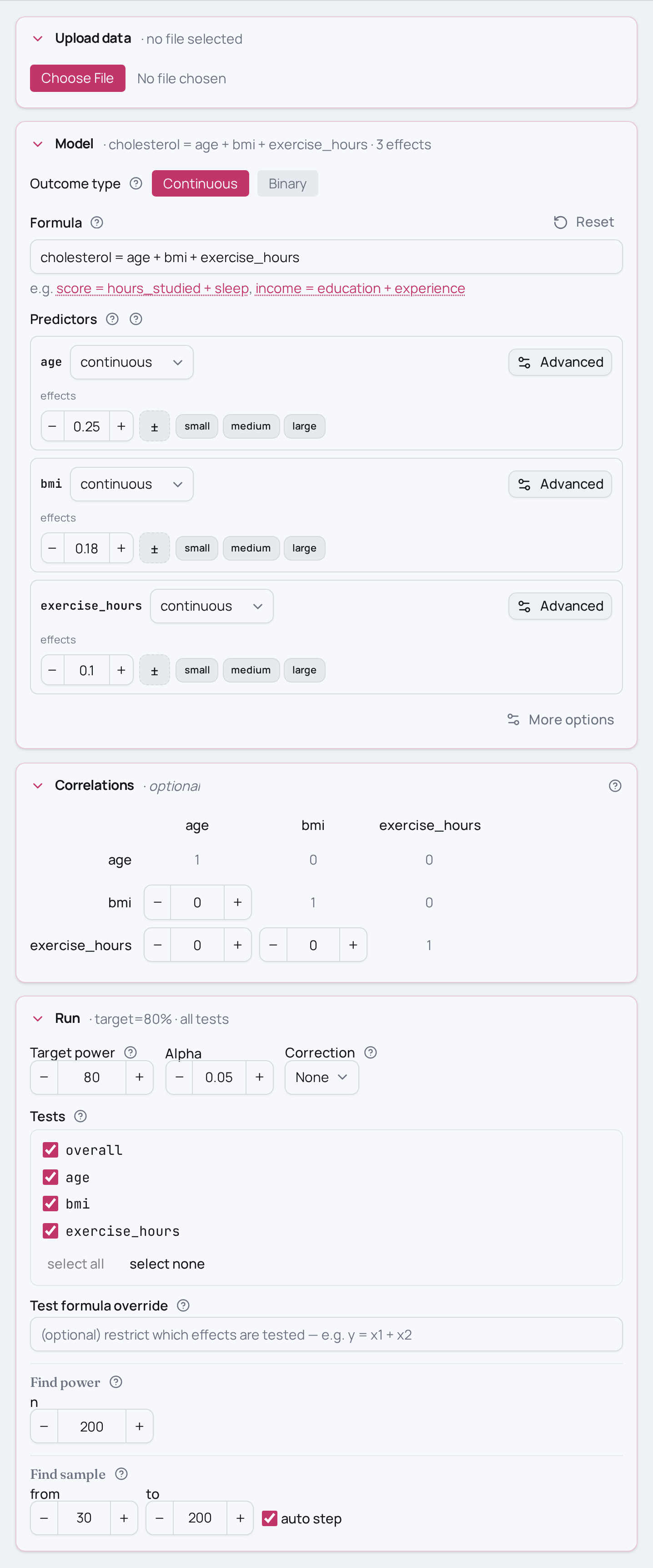
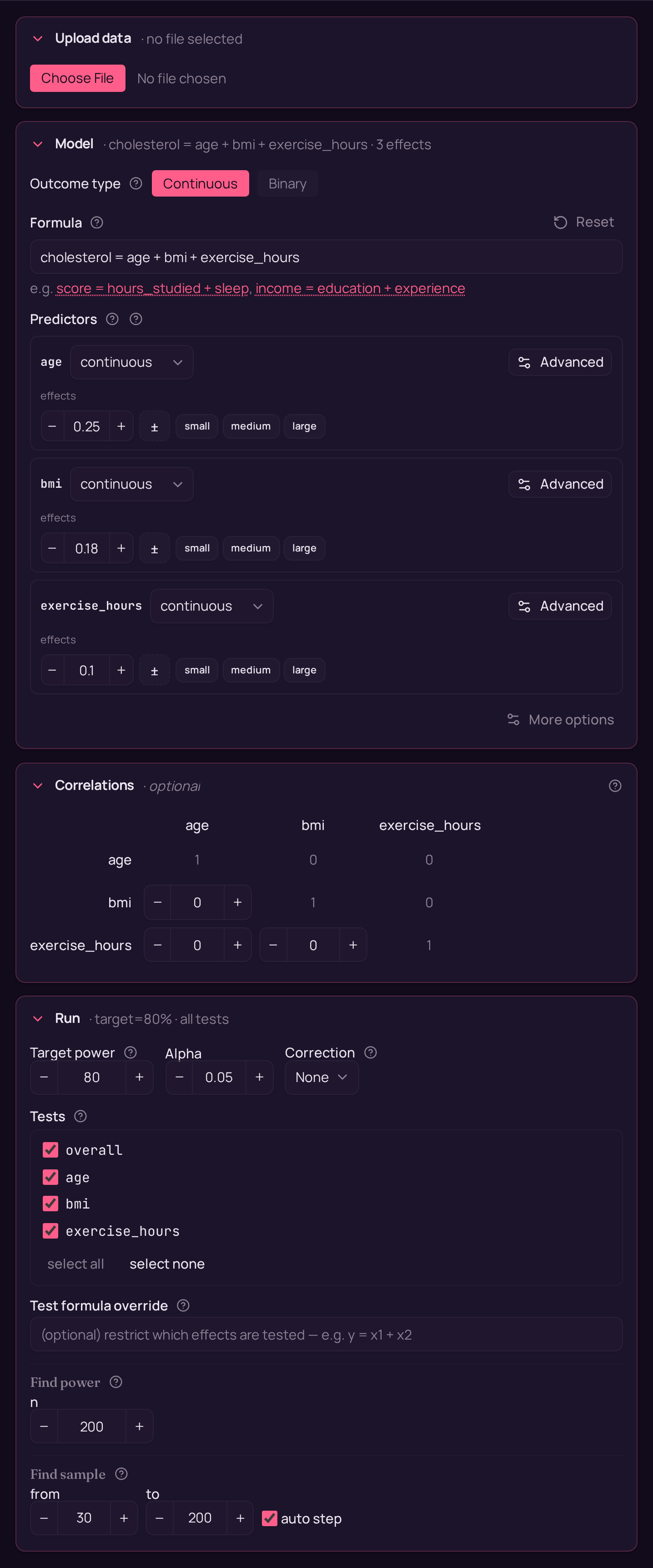
Do age, BMI, and weekly exercise hours each independently predict cholesterol once the others are held constant? Three continuous predictors entered together — no groups, no interactions, just parallel main effects. As an MCPower formula this is cholesterol ~ age + bmi + exercise_hours: an OLS model with three additive continuous slopes.

Variations

• More or fewer predictors. Drop exercise_hours for a two-predictor model, or keep adding terms (+ blood_pressure + biomarker_level) — give each a name and an effect size and the setup is unchanged.
• Different effect-size mix. The numbers here are standardised slopes on the continuous benchmark scale (small 0.10, medium 0.25, large 0.40); set each predictor to whatever you expect, e.g. age=0.40, bmi=0.10, exercise_hours=0.10.
• Find the N instead of the power. Swap find_power(sample_size=200, …) for find_sample_size(target_test="age, bmi, exercise_hours", from_size=50, to_size=400) to get the smallest N that reaches 80% power.
• Correlated predictors. If your three measures are themselves related, add set_correlations("corr(age, bmi)=0.3") — collinearity drains power, so it is worth modelling.
• Same design, other fields:
  • Ecology: plant_biomass ~ rainfall + soil_nitrogen + temperature — three environmental drivers of biomass; same additive three-predictor OLS shape.
  • Social: wage ~ years_education + experience_years + tenure — three continuous predictors of wage; same formula structure.

Not this setup?

• Two continuous predictors — the same additive shape with one fewer term.
• Many continuous covariates — when the predictor list grows beyond a handful.
• A single continuous predictor — the plain simple-regression case, one slope only.

If you'd rather have…

• Two predictors that interact (moderation) — let two of your continuous predictors interact instead of just adding them.
• A full three-way interaction — go further to a three-way interaction among three continuous predictors.
• A binary plus continuous predictors — swap one continuous predictor for a binary one (mixed binary + continuous, parallel slopes).
• An interaction plus a control covariate — keep a continuous interaction but add a separate covariate as a control.

Copy-paste setup

from mcpower import MCPower

# Three continuous predictors, additive (no interactions): each contributes
# independently to the outcome on the standardised effect scale.
model = MCPower("cholesterol = age + bmi + exercise_hours")

# Standardised slopes: age medium (0.25), bmi small-to-medium (0.18), exercise_hours small (0.10).
model.set_effects("age=0.25, bmi=0.18, exercise_hours=0.10")

model.set_seed(2137)
model.set_simulations(1600)

model.find_power(sample_size=200, target_test="age, bmi, exercise_hours")

suppressMessages(library(mcpower))

# Three continuous predictors, additive (no interactions): each contributes
# independently to the outcome on the standardised effect scale.
model <- MCPower$new("cholesterol ~ age + bmi + exercise_hours")

# Standardised slopes: age medium (0.25), bmi small-to-medium (0.18), exercise_hours small (0.10).
model$set_effects("age=0.25, bmi=0.18, exercise_hours=0.10")

model$set_seed(2137)
model$set_simulations(1600)

invisible(model$find_power(sample_size = 200, target_test = "age, bmi, exercise_hours"))