Power analysis for simple linear regression

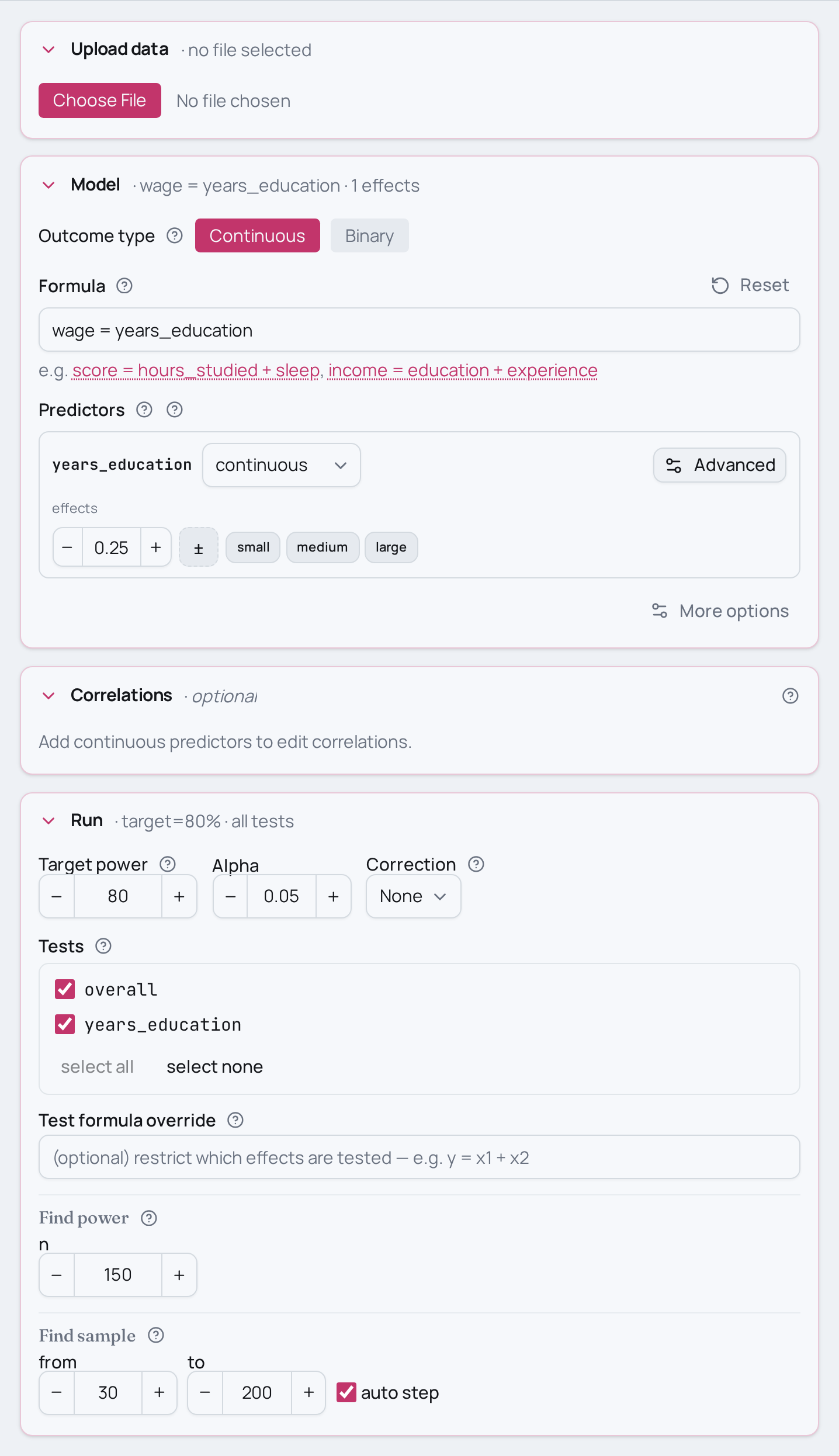
Does years of education predict wage? The simplest regression structure: one continuous outcome regressed on one continuous predictor, nothing held constant. As an MCPower formula this is wage ~ years_education: one predictor, no covariates, no interactions.

Variations

• Dial the expected association up or down by changing the effect: years_education=0.10 for a small relationship, years_education=0.40 for a large one (the medium benchmark is 0.25).
• Searching for the sample size that reaches 80% power instead of scoring a fixed N? Swap find_power(sample_size=150, ...) for find_sample_size(target_test="years_education", from_size=30, to_size=300, by=10).
• Same design, other fields:
  • Clinical: pain_score ~ dose_level — linear trend of pain score across an escalating drug dose; same single-predictor OLS structure.
  • Ecology: plant_biomass ~ rainfall — does annual rainfall predict plant biomass across sites? Same formula shape, continuous environmental predictor.

Not this setup?

• Add a binary group alongside the continuous predictor (parallel slopes)
• Two continuous predictors (wage ~ years_education + experience_years)
• Binary group instead of a continuous predictor
• Ordinal / dose predictor read as a linear trend

If you'd rather have…

• Multiple regression — add a second continuous predictor (wage ~ years_education + experience_years) for multiple regression.
• Moderation between two predictors — let two continuous predictors interact (wage ~ years_education * experience_years) to test moderation.
• Independent t-test as regression — use a binary group instead of a continuous predictor.
• Linear trend across a dose — treat an ordinal/dose predictor as continuous to test a linear trend.
• Adjusted association with covariates — estimate one exposure's adjusted association while controlling for several covariates.

Copy-paste setup

from mcpower import MCPower

# Simple linear regression: one continuous outcome, one continuous predictor.
model = MCPower("wage = years_education")

# Expected effect on the standardised benchmark scale:
#   years_education=0.25 -> a medium association between years_education and wage.
model.set_effects("years_education=0.25")

# Power at N=150 with the OLS defaults (1600 sims, alpha=0.05, seed=2137).
model.find_power(sample_size=150, target_test="years_education")

suppressMessages(library(mcpower))

# Simple linear regression: one continuous outcome, one continuous predictor.
model <- MCPower$new("wage ~ years_education")

# Expected effect on the standardised benchmark scale:
#   years_education=0.25 -> a medium association between years_education and wage.
model$set_effects("years_education=0.25")

# Power at N=150 with the OLS defaults (1600 sims, alpha=0.05, seed=2137).
invisible(model$find_power(sample_size = 150, target_test = "years_education"))