Power analysis for a linear dose-response trend

You ran a study with an ordered dose — a placebo and three escalating treatment levels coded 0, 1, 2, 3 — and measured tumor_shrinkage as a continuous outcome. Rather than asking whether any one level differs from another, you want the power to detect a steady linear-by-level trend: as dose_level climbs from 0 to 3, does tumor shrinkage move with it? Treating the dose as a single numeric predictor turns that question into one slope.

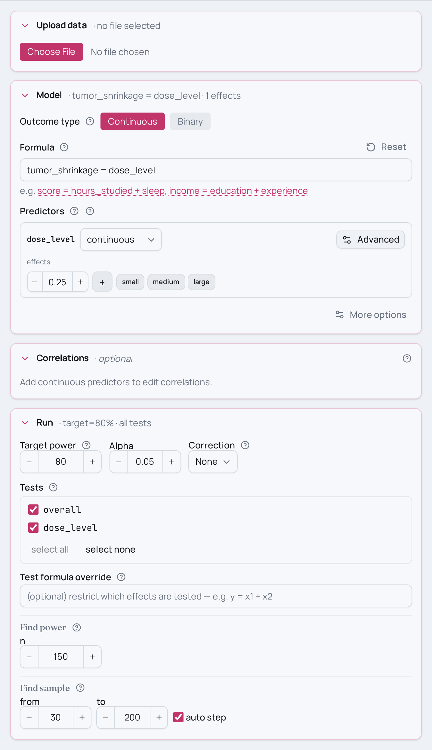
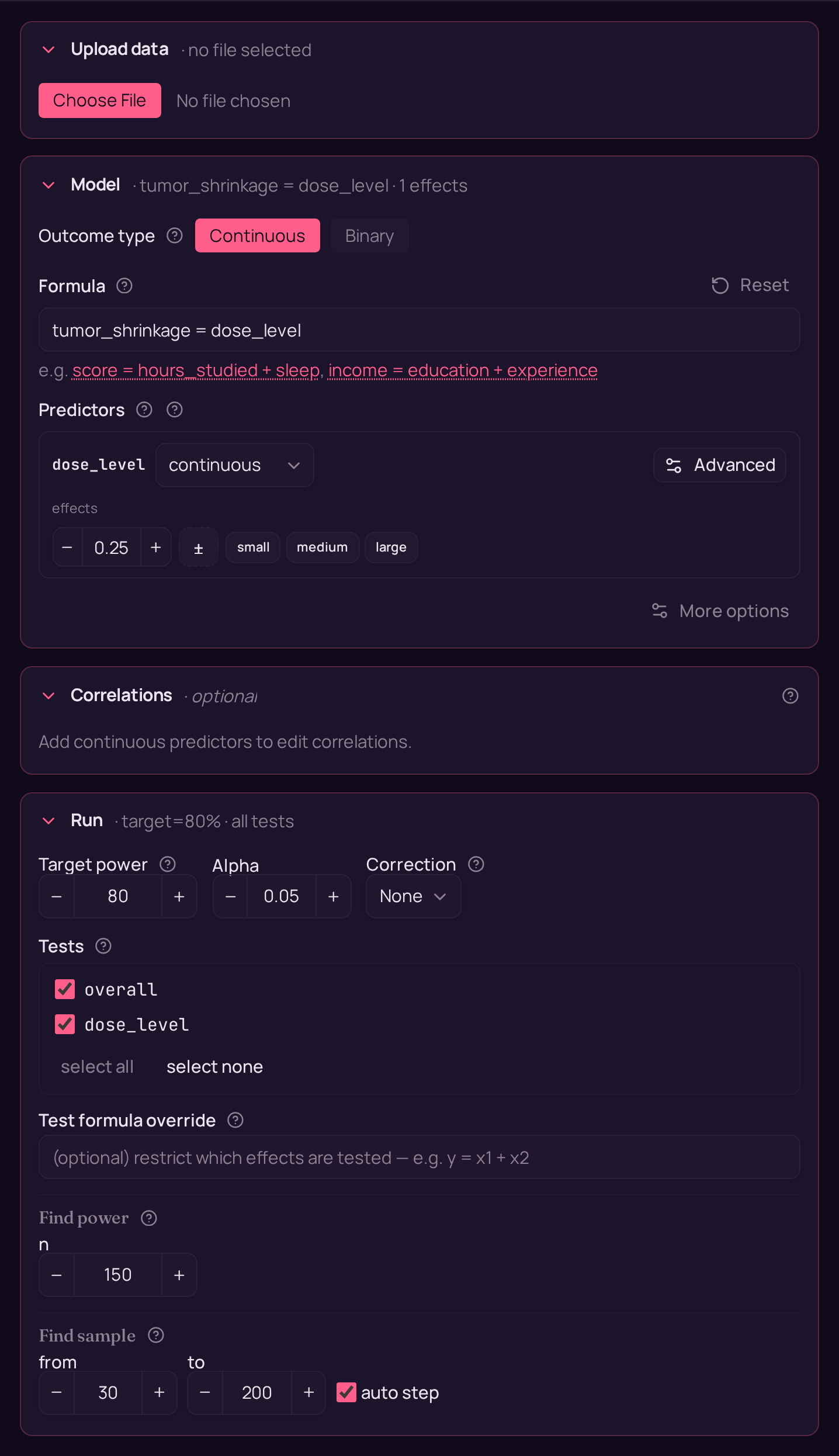
As an MCPower model this is tumor_shrinkage = dose_level, where dose_level is read as a continuous predictor — one coefficient, no covariates, no interactions — and the reported power is the power to detect that single trend.

Variations

• Dial the expected trend up or down. Change the effect: dose_level=0.10 for a shallow slope, dose_level=0.40 for a steep one (the medium benchmark is 0.25).
• Treat the dose levels as an unordered categorical factor. Swap dose_level for dose_level=(factor,4) to dummy-code each level against a reference rather than fitting one slope.
• Find the N instead of scoring a fixed sample. Swap find_power(sample_size=150, ...) for find_sample_size(target_test="dose_level", from_size=30, to_size=300, by=10) to search for the smallest N that reaches 80% power.
• Same design, other fields:
  • Ecology: plant_biomass ~ nitrogen — does plant biomass increase linearly with nitrogen application level (0–3)?
  • Social science: well_being ~ social_support — does well-being increase linearly across levels of a social support index?

Not this setup?

• One continuous predictor, no dose structure (wage ~ years_education)
• Dose levels as an unordered factor, not a trend
• Two groups instead of a graded dose

If you'd rather have…

• Dose levels as a categorical factor — treat the dose levels as an unordered categorical factor (dummy-coded) instead of a linear trend, testing each level against a reference rather than a single slope.
• Omnibus test across dose groups — test for any difference across dose groups with an omnibus ANOVA instead of a linear-by-level trend.
• Add a second continuous predictor — add a second continuous predictor (e.g. a covariate) to the dose trend for a multiple-regression adjustment.
• ANCOVA-style covariate adjustment — adjust the dose effect for a baseline covariate in an ANCOVA-style design.

Copy-paste setup

from mcpower import MCPower

# Linear dose-response: one continuous outcome regressed on an ordered dose level.
# The dose_level values (0, 1, 2, 3, ...) are read as a single continuous predictor,
# so the test is one slope -- a linear-by-level trend across the dose.
model = MCPower("tumor_shrinkage = dose_level")

# Expected effect on the standardised benchmark scale:
#   dose_level=0.25 -> a medium linear trend of the outcome across the dose levels.
model.set_effects("dose_level=0.25")

# Power at N=150 with the OLS defaults (1600 sims, alpha=0.05, seed=2137).
model.find_power(sample_size=150, target_test="dose_level")

suppressMessages(library(mcpower))

# Linear dose-response: one continuous outcome regressed on an ordered dose level.
# The dose_level values (0, 1, 2, 3, ...) are read as a single continuous predictor,
# so the test is one slope -- a linear-by-level trend across the dose.
model <- MCPower$new("tumor_shrinkage ~ dose_level")

# Expected effect on the standardised benchmark scale:
#   dose_level=0.25 -> a medium linear trend of the outcome across the dose levels.
model$set_effects("dose_level=0.25")

# Power at N=150 with the OLS defaults (1600 sims, alpha=0.05, seed=2137).
invisible(model$find_power(sample_size = 150, target_test = "dose_level"))