Power analysis for a logistic GLMM with random slope
You resurveyed the same sites repeatedly across a temperature gradient and
recorded whether the target species was detected (yes/no). You expect not just
different baseline detection rates between sites but different temperature
responses — some sites show sharp presence-absence thresholds with temperature,
others barely respond — so you fit a logistic mixed model with a random intercept
and a random slope of temperature per site:
species_present ~ temperature + (1 + temperature|site).
Variations
- Drop the random slope. Change the formula to
species_present ~ temperature + (1|site)and removerandom_slopes,slope_variance, andslope_intercept_corrfromset_clusterif you only expect sites to differ in baseline detection rate, not in how they respond to temperature. A fixed slope is cheaper to power but overstates power when the slope really does vary. - More or less slope spread.
slope_variance=0.15is the spread of per-site temperature slopes; push it toward0.30(sites respond very differently) or0.05(nearly parallel responses). More slope spread widens the standard error of the average temperature effect and costs power. - Stronger or weaker clustering.
ICC=0.10says 10% of the baseline variance sits between sites. Raise it towardICC=0.30to leave less independent information per observation. - More sites vs more observations. Hold N=400 but change
n_clusters— 20 sites means 20 observations each, 80 means 5 each. Adding sites usually buys more power for a slope than adding observations to the same sites. - Smaller or larger temperature effect.
temperature=0.25is a medium association on the continuous benchmark scale; swap it fortemperature=0.10(small) ortemperature=0.40(large). - Solve for N instead. Replace
find_power(sample_size=400, …)withfind_sample_size(target_test="temperature", from_size=200, to_size=800, by=100)to get the minimum total sample that reaches 80% power. - Same design, other fields
- Clinical:
remission ~ dose + (1 + dose|patient)— remission status (yes/no) recorded at multiple dose levels per patient, where each patient has their own dose-response slope. - Social science:
employed ~ experience_years + (1 + experience_years|region)— employment status (yes/no) across individuals in multiple regions, where each region's experience-employment gradient is allowed to vary.
- Clinical:
Not this setup?
- Longitudinal binary outcome with a random intercept — same binary
GLMM family but only a random intercept per patient (
(1|patient)), no random slope. - Cluster-randomised binary trial — the simplest binary mixed
model: a random intercept per cluster (
(1|cluster)) and no random slope. - Random intercept and slope, continuous outcome — the same
intercept-and-slope structure (
(time|participant)) but with a continuous outcome instead of binary.
If you'd rather have…
- Longitudinal binary outcome — longitudinal binary outcome with a
random intercept per patient (
symptom_present ~ month + treatment + (1|patient)) — same binary GLMM family but only a random intercept, no random slope. - Cluster-randomised binary GLMM — cluster-randomised binary GLMM
with just a random intercept (
infection ~ treatment + (1|hospital)) — the simplest binary mixed model, drop the random slope. - Random intercept and slope — same random-intercept-and-slope-of-a-
continuous-predictor structure (
(time|participant)) but with a continuous (Gaussian) outcome instead of binary. - Simple logistic regression — logistic regression of a binary outcome on one continuous predictor — the single-level (no random effects) version of this design.
- Random slope across clusters — random slope of a predictor across
clusters (
(treatment|site)) — the random-slope idea on a continuous outcome with a treatment predictor.
Copy-paste setup
from mcpower import MCPower
# Species presence (yes/no) recorded repeatedly across temperature gradients at
# the same sites, where each site responds to temperature at its own rate.
# family="logit" makes species_present binary (fit by GLM); (1 + temperature|site)
# adds a random intercept AND a random slope of temperature per site, so the
# average temperature effect is tested with the extra site-to-site slope spread
# folded into its standard error.
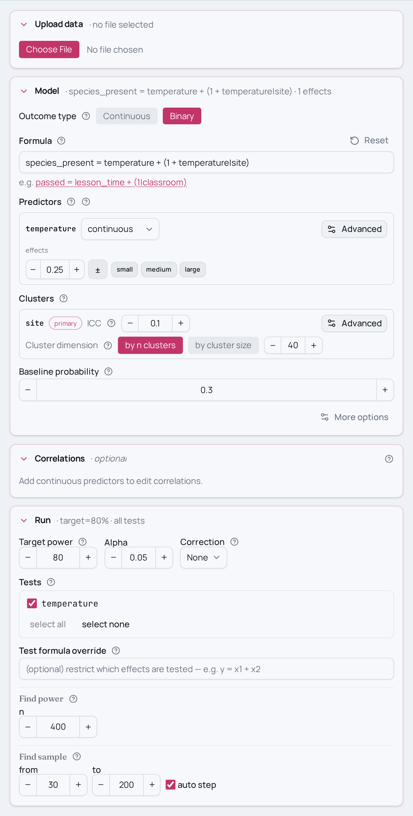
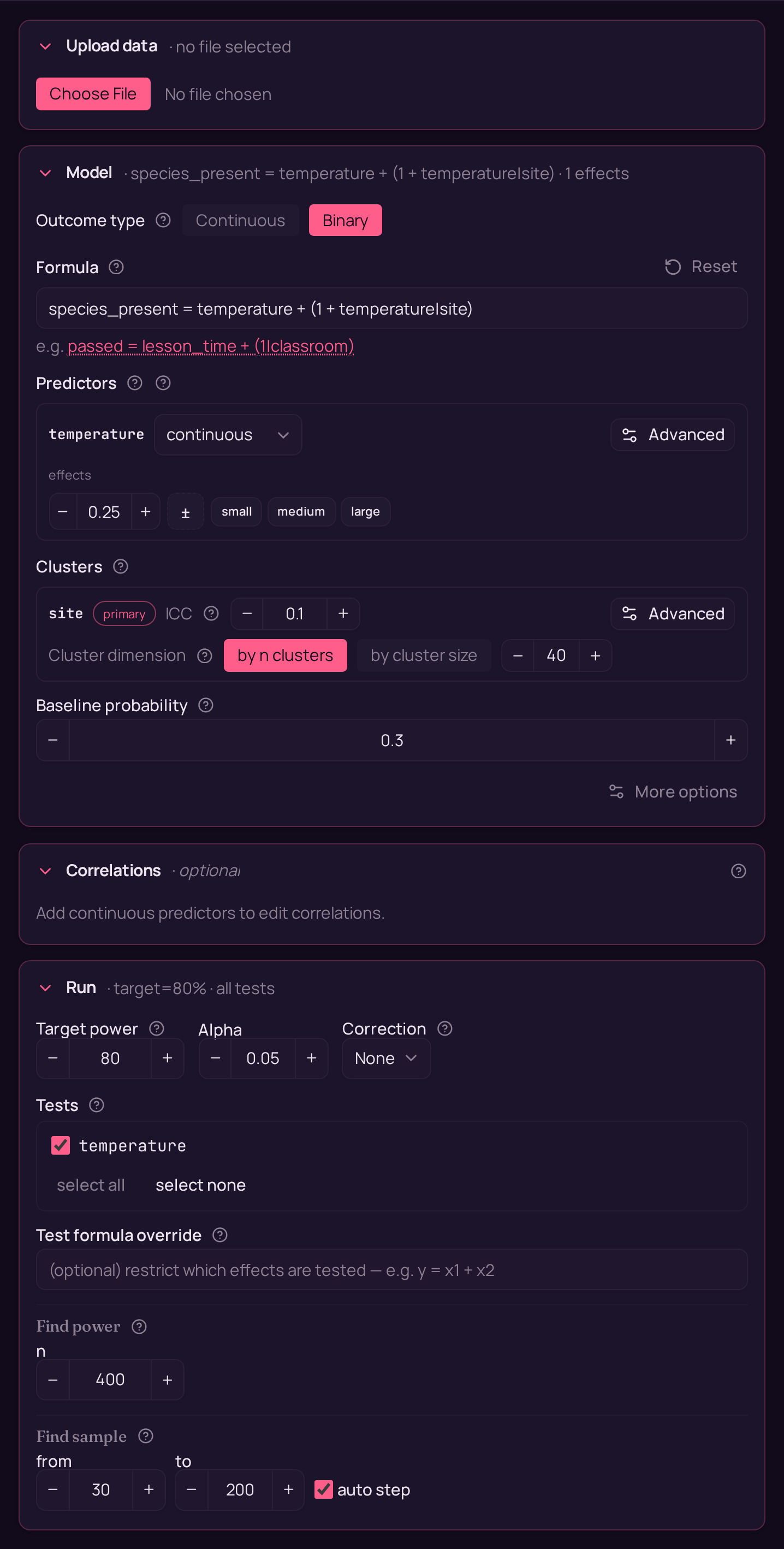
model = MCPower("species_present = temperature + (1 + temperature|site)", family="logit")
# Binary outcome needs its no-predictor base rate: 30% of surveys detect the
# species when temperature is at its average.
model.set_baseline_probability(0.3)
# Expected effect on the standardised benchmark scale (continuous predictor):
# temperature=0.25 -> a medium association with the log-odds of species presence.
model.set_effects("temperature=0.25")
# Clustering: ICC=0.10 between sites across 40 sites. random_slopes names the
# predictor whose slope varies; slope_variance is the spread of those per-site
# temperature slopes and slope_intercept_corr their correlation with the random
# intercept. At N=400 that is 10 observations per site.
model.set_cluster("site", ICC=0.10, n_clusters=40,
random_slopes=["temperature"], slope_variance=0.15,
slope_intercept_corr=0.0)
# Power at N=400 for the average temperature effect (GLM defaults: 1600 sims,
# alpha=0.05, seed=2137). The omnibus test is not reported for mixed models;
# target the coefficient directly.
model.find_power(sample_size=400, target_test="temperature")
suppressMessages(library(mcpower))

# Species presence (yes/no) recorded repeatedly across temperature gradients at
# the same sites, where each site responds to temperature at its own rate.
# family = "logit" makes species_present binary (fit by GLM); (1 + temperature|site)
# adds a random intercept AND a random slope of temperature per site, so the
# average temperature effect is tested with the extra site-to-site slope spread
# folded into its standard error.
model <- MCPower$new("species_present ~ temperature + (1 + temperature|site)", family = "logit")

# Binary outcome needs its no-predictor base rate: 30% of surveys detect the
# species when temperature is at its average.
model$set_baseline_probability(0.3)

# Expected effect on the standardised benchmark scale (continuous predictor):
#   temperature=0.25 -> a medium association with the log-odds of species presence.
model$set_effects("temperature=0.25")

# Clustering: ICC=0.10 between sites across 40 sites. random_slopes is a list
# of one spec per random slope; each names the predictor whose slope varies
# (variance = the spread of those per-site temperature slopes, corr_with_intercept =
# their correlation with the random intercept). At N=400 that is 10 observations
# per site.
model$set_cluster("site", ICC = 0.10, n_clusters = 40,
                  random_slopes = list(
                    list(predictor = "temperature", variance = 0.15,
                         corr_with_intercept = 0.0)
                  ))

# Power at N=400 for the average temperature effect (GLM defaults: 1600 sims,
# alpha=0.05, seed=2137). The omnibus test is not reported for mixed models;
# target the coefficient directly.
invisible(model$find_power(sample_size = 400, target_test = "temperature"))