Power analysis for a longitudinal binary outcome

You ran a two-arm study (control vs. treatment) and recorded whether a symptom was present — a binary outcome (yes/no) — at several months on the same patients. You want to know whether the symptom becomes more or less likely over time and whether the two arms differ. 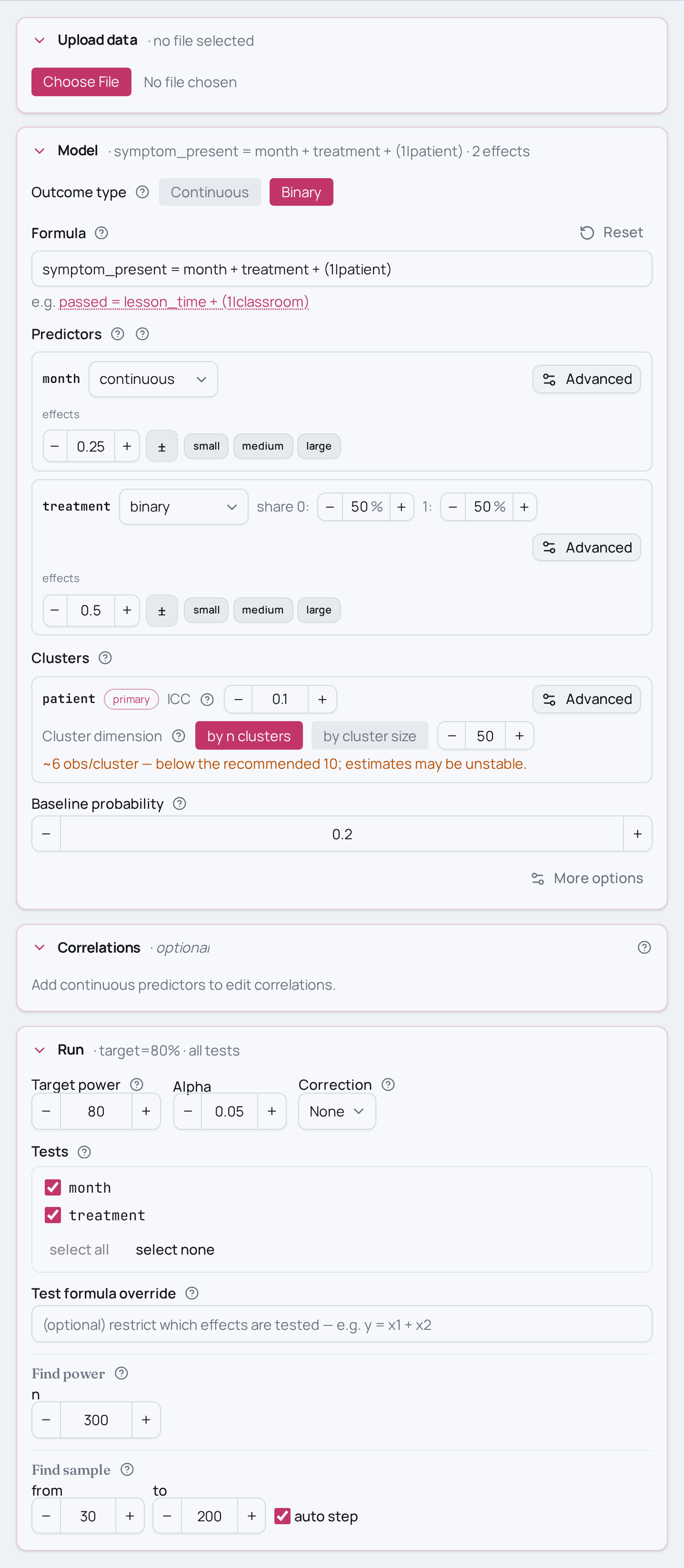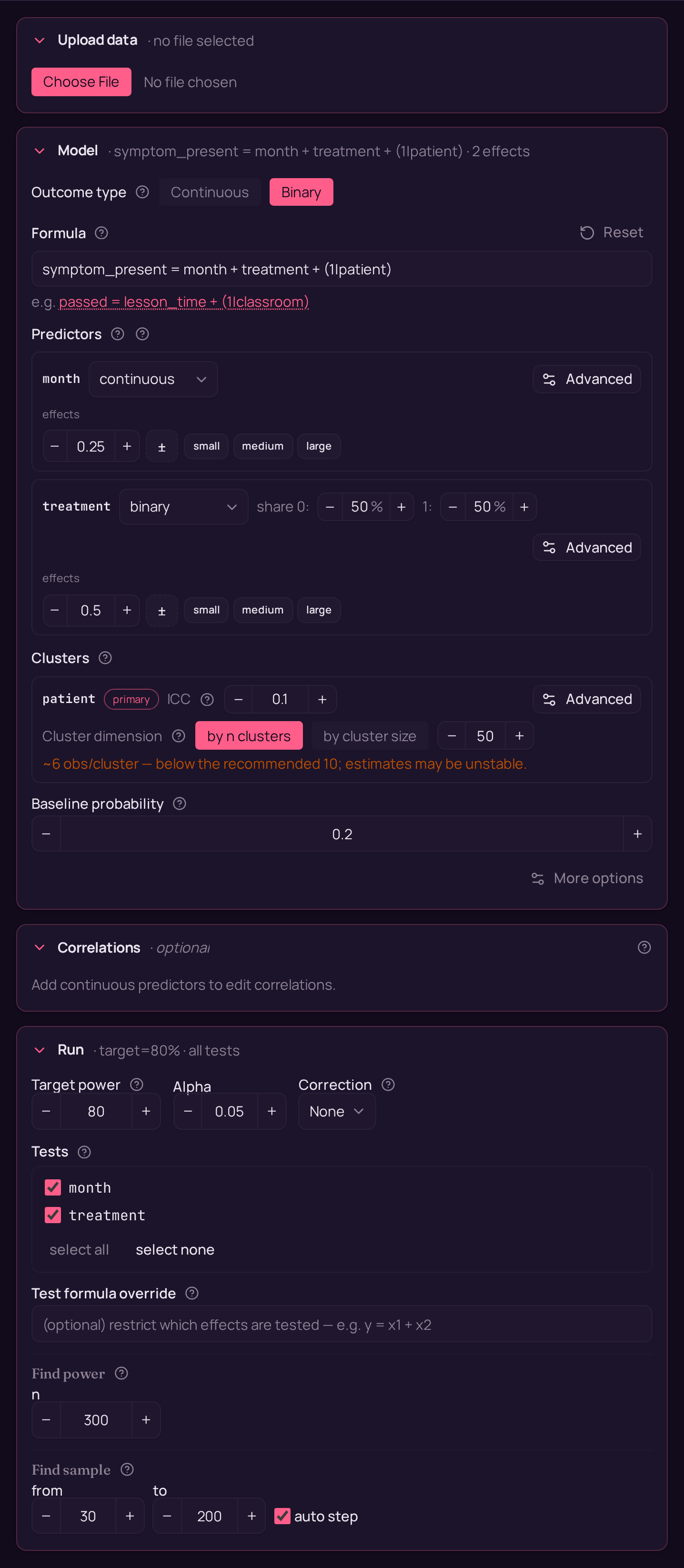Because the repeated measurements on one patient are correlated, you fit a binary generalised linear mixed model with a random intercept per patient: symptom_present ~ month + treatment + (1|patient).

Variations

• Stronger or weaker clustering. The ICC=0.10 in set_cluster says 10% of the latent variance sits between patients. Push it toward ICC=0.05 (patients behave almost interchangeably) or ICC=0.30 (patients differ a lot) — higher ICC leaves less independent information per measurement and costs power for the same N.
• More patients vs more measurements. Hold N=300 but change n_clusters — 30 patients means 10 measurements each, 75 means 4 each. Adding patients usually buys more power than adding measurements to the same patients.
• A rarer or commoner symptom. set_baseline_probability(0.20) is the control symptom rate at baseline; drop it to 0.05 (rare symptoms are hard to detect) or raise it toward 0.40 to see how the base rate moves power.
• Smaller or larger effects. treatment=0.50 and month=0.25 are medium on the binary benchmark scale; swap in treatment=0.20 / month=0.10 (small) or treatment=0.80 / month=0.40 (large) to see how the expected gap and slope move power.
• Solve for N instead. Replace find_power(sample_size=300, …) with find_sample_size(target_test="month, treatment", from_size=180, to_size=600, by=60) to get the minimum total sample that reaches 80% power.
• Same design, other fields
  • Ecology: germinated ~ month + treatment + (1|seedling) — seedling germination (yes/no) recorded at monthly intervals across two irrigation regimes, with each seedling as its own cluster.
  • Social science: employed ~ period + treatment + (1|individual) — employment status (yes/no) tracked over several survey periods for individuals in a job-placement programme vs control.

Not this setup?

• Difference-in-differences (group x time interaction)
• Clustered binary outcome with one treatment effect
• Two arms over time on a continuous outcome

If you'd rather have…

• Group x time interaction — same binary longitudinal design with a random intercept per patient, but add the group x time interaction (difference-in-differences) instead of parallel main effects.
• Simpler binary GLMM — one fixed effect (treatment) with a random intercept per cluster, no time dimension.
• Continuous two-arm longitudinal — same two-arm random-intercept-per-participant structure, but for a continuous outcome and with a treatment x time interaction.
• Random slope — step up the random structure: a binary outcome with a random slope (temperature | site) rather than a random intercept only.
• Continuous repeated measures — the continuous-outcome analogue of a basic longitudinal repeated-measures design with a random intercept per participant.
• Single-level logistic comparison — drop the clustering entirely: a two-group logistic comparison if patients aren't measured repeatedly.

Copy-paste setup

from mcpower import MCPower

# Longitudinal binary outcome: symptom presence (yes/no) recorded at several
# months on the same patients, in two arms (control vs. treatment). The
# (1|patient) term adds a random intercept per patient; family="logit" with a
# cluster makes this a binary GLMM (GLM estimator).
model = MCPower("symptom_present = month + treatment + (1|patient)", family="logit")

# treatment is a binary two-level predictor (0 = control, 1 = treatment); month
# is continuous (measurement occasion on the standardised benchmark scale).
model.set_variable_type("treatment=binary")

# Expected effects on the binary benchmark scale:
#   treatment=0.50 -> a medium gap between arms,
#   month=0.25     -> a medium change in symptom odds per month.
model.set_effects("treatment=0.50, month=0.25")

# Symptom rate in the control group at baseline (logit family needs one).
model.set_baseline_probability(0.20)

# Describe the clustering: ICC=0.10 (10% of the latent variance is between
# patients) across 50 patients. At N=300 that is 6 measurements each.
model.set_cluster("patient", ICC=0.10, n_clusters=50)

# Power at N=300 for both fixed effects (mixed defaults: 800 sims, alpha=0.05,
# seed=2137). The omnibus test is not reported for mixed models; target the
# coefficients directly.
model.find_power(sample_size=300, target_test="month, treatment")

suppressMessages(library(mcpower))

# Longitudinal binary outcome: symptom presence (yes/no) recorded at several
# months on the same patients, in two arms (control vs. treatment). The
# (1|patient) term adds a random intercept per patient; family = "logit" with a
# cluster makes this a binary GLMM (GLM estimator).
model <- MCPower$new("symptom_present ~ month + treatment + (1|patient)", family = "logit")

# treatment is a binary two-level predictor (0 = control, 1 = treatment); month
# is continuous (measurement occasion on the standardised benchmark scale).
model$set_variable_type("treatment=binary")

# Expected effects on the binary benchmark scale:
#   treatment=0.50 -> a medium gap between arms,
#   month=0.25     -> a medium change in symptom odds per month.
model$set_effects("treatment=0.50, month=0.25")

# Symptom rate in the control group at baseline (logit family needs one).
model$set_baseline_probability(0.20)

# Describe the clustering: ICC=0.10 (10% of the latent variance is between
# patients) across 50 patients. At N=300 that is 6 measurements each.
model$set_cluster("patient", ICC = 0.10, n_clusters = 50)

# Power at N=300 for both fixed effects (mixed defaults: 800 sims, alpha=0.05,
# seed=2137). The omnibus test is not reported for mixed models; target the
# coefficients directly.
invisible(model$find_power(sample_size = 300, target_test = "month, treatment"))