Power analysis for a binary difference-in-differences

You tracked individuals across several periods and recorded whether each was employed (yes/no). A policy_group indicator is crossed with period, and the question is not either main effect but whether the two groups change differently: does the policy group's employment trajectory diverge from the control group's? That is the classic difference-in-differences (DiD), the group-by-period interaction — here on the log-odds scale, because the outcome is binary, and with a random intercept per individual, because the repeated observations on one person are correlated.

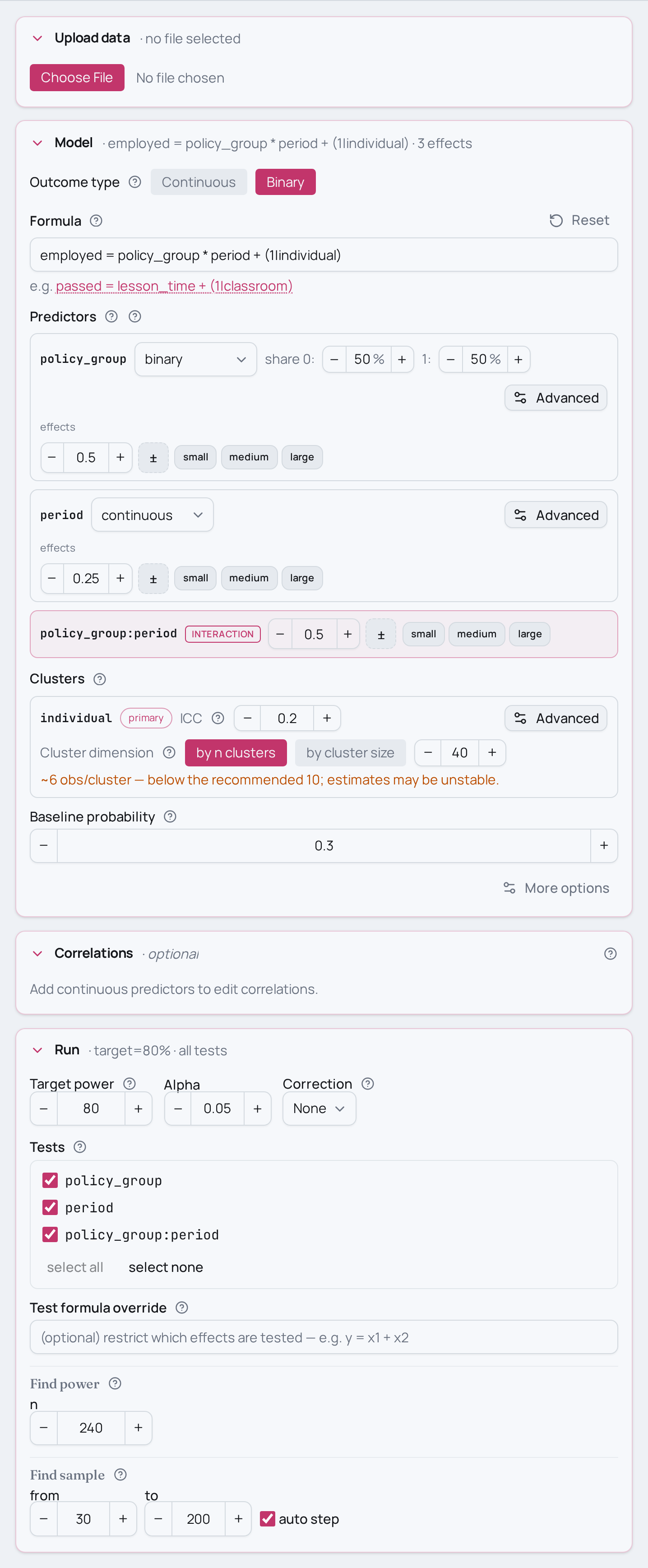
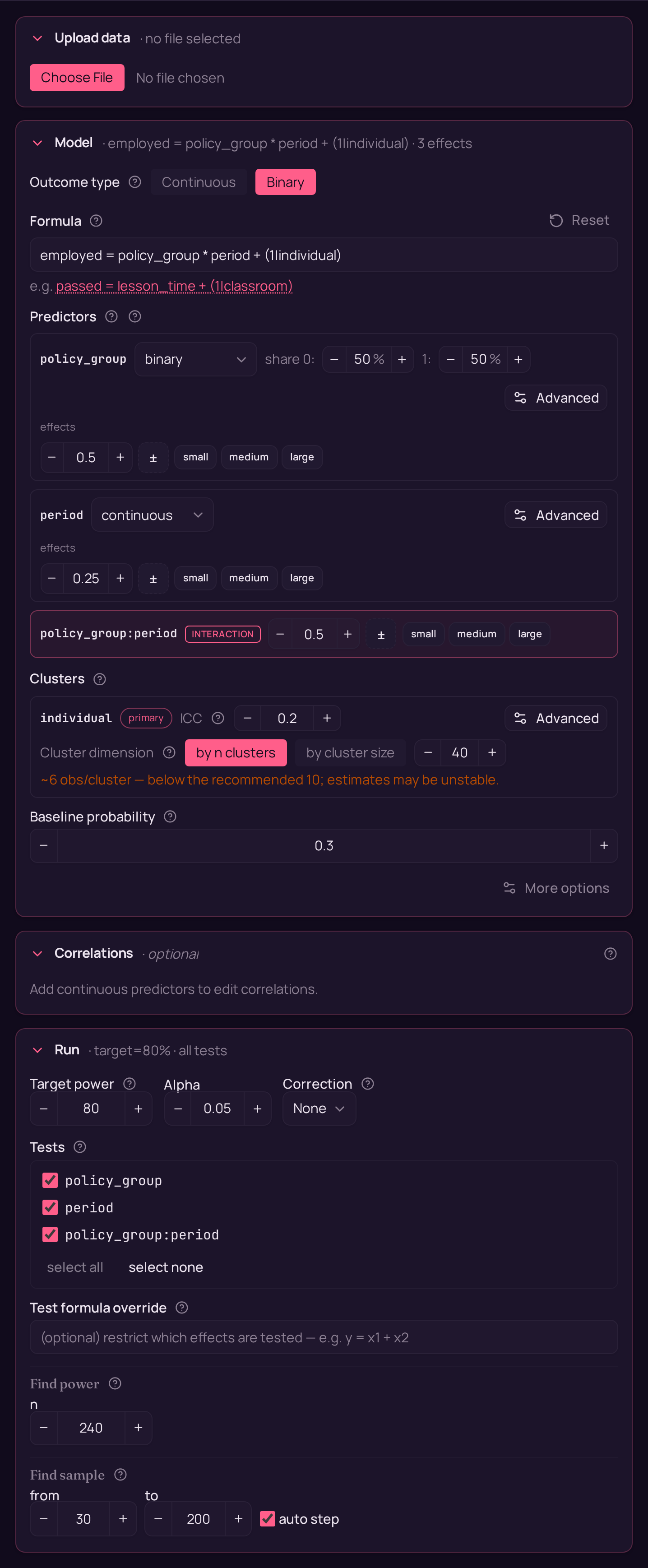
As an MCPower formula this is employed = policy_group * period + (1|individual) with family="logit", where * expands to policy_group + period + policy_group:period. policy_group is a two-level binary predictor and period is continuous; the test of interest is the interaction term policy_group:period, fitted as a logistic mixed model (GLMM).

Variations

Stronger or weaker clustering. The ICC=0.20 in set_cluster says 20% of the latent variance sits between individuals. Push it toward ICC=0.05 (individuals are nearly interchangeable) or ICC=0.40 (individuals differ a lot) — higher ICC leaves less independent information per observation and costs power for the same N.
More individuals vs more observations. Hold N=240 but change n_clusters — 24 individuals means 10 observations each, 60 means 4 each. Adding individuals usually buys more power for a between-group contrast than adding observations to the same people.
Stronger or weaker policy effect. policy_group:period=0.50 is a medium DiD on the factor benchmark scale; swap it for policy_group:period=0.20 (subtle divergence) or policy_group:period=0.80 (the groups respond very differently) to watch how fast power for the interaction collapses as the effect shrinks.
Solve for N instead. Replace find_power(sample_size=240, …) with find_sample_size(target_test="policy_group:period", from_size=160, to_size=640, by=40) to get the minimum total sample that reaches 80% power. A logistic interaction on clustered binary data needs markedly more N than either main effect, so set the upper bound generously.
Same design, other fields
- Clinical: remission ~ treatment * month + (1|patient) — remission status (yes/no) tracked over months in a clinical trial, testing whether the treatment group's remission trajectory diverges from the control group's.
- Ecology: survived ~ habitat * period + (1|seedling) — seedling survival (yes/no) across two habitat types measured at several time points, testing whether survival trajectories diverge between habitat types.

Not this setup?

If you'd rather have…

Treatment x time interaction (two-arm longitudinal / split-plot mixed ANOVA) — Same treatment-by-time interaction with a random intercept, but on a continuous (Gaussian) outcome instead of binary — the DiD design for a measured response.
Longitudinal binary outcome over time (random intercept per patient) — Same longitudinal binary outcome and random intercept per patient, but additive group + time (no interaction) — main effects of time and group rather than a difference-in-differences.
Logistic factor-by-factor interaction (2x2) — Same group-by-time-style 2x2 interaction on a binary outcome, but with no random effect — a plain logistic factorial when measurements are independent rather than repeated.
Logistic GLMM with a continuous predictor and random slope — Binary GLMM where the predictor effect varies across subjects (random slope) instead of a fixed interaction with a random intercept.

Copy-paste setup

from mcpower import MCPower

# Difference-in-differences on a binary employment outcome: each individual is
# observed at several periods, and we record whether they are `employed` (yes/no).
# A policy `policy_group` is crossed with `period` — the question is whether the
# change over periods differs between groups (the DiD interaction). '*' expands
# policy_group * period to policy_group + period + policy_group:period, so the
# interaction is fitted explicitly, on the log-odds scale. family="logit" makes
# employed binary (0/1); the (1|individual) random intercept makes it a logistic
# GLMM, fitted by the GLM estimator.
model = MCPower("employed = policy_group * period + (1|individual)", family="logit")

# policy_group is a two-level factor (policy vs control); period is the
# continuous measurement occasion.
model.set_variable_type("policy_group=binary")

# Effect sizes on the relevant benchmark scales, each a shift in the log-odds of
# being employed:
#   policy_group=0.50             -> medium baseline arm difference (factor benchmark).
#   period=0.25                   -> medium average change over time (continuous benchmark).
#   policy_group:period=0.50      -> medium DiD interaction: the policy group's
#                                    trajectory diverges from the control group's
#                                    (factor benchmark).
model.set_effects("policy_group=0.50, period=0.25, policy_group:period=0.50")

# Baseline employment rate of 30% when all predictors are at their reference.
model.set_baseline_probability(0.30)

# Clustering: ICC=0.20 (20% of the latent variance is between individuals)
# across 40 individuals. At N=240 that is 6 observations per individual.
model.set_cluster("individual", ICC=0.20, n_clusters=40)

# Power at N=240 for the DiD interaction (mixed defaults: 800 sims, alpha=0.05,
# seed=2137). The omnibus test is not reported for mixed models; target the
# interaction coefficient directly.
model.find_power(sample_size=240, target_test="policy_group:period")

suppressMessages(library(mcpower))

# Difference-in-differences on a binary employment outcome: each individual is
# observed at several periods, and we record whether they are `employed` (yes/no).
# A policy `policy_group` is crossed with `period` — the question is whether the
# change over periods differs between groups (the DiD interaction). '*' expands
# policy_group * period to policy_group + period + policy_group:period, so the
# interaction is fitted explicitly, on the log-odds scale. family = "logit" makes
# employed binary (0/1); the (1|individual) random intercept makes it a logistic
# GLMM, fitted by the GLM estimator.
model <- MCPower$new("employed ~ policy_group * period + (1|individual)", family = "logit")

# policy_group is a two-level factor (policy vs control); period is the
# continuous measurement occasion.
model$set_variable_type("policy_group=binary")

# Effect sizes on the relevant benchmark scales, each a shift in the log-odds of
# being employed:
#   policy_group=0.50             -> medium baseline arm difference (factor benchmark).
#   period=0.25                   -> medium average change over time (continuous benchmark).
#   policy_group:period=0.50      -> medium DiD interaction: the policy group's
#                                    trajectory diverges from the control group's
#                                    (factor benchmark).
model$set_effects("policy_group=0.50, period=0.25, policy_group:period=0.50")

# Baseline employment rate of 30% when all predictors are at their reference.
model$set_baseline_probability(0.30)

# Clustering: ICC=0.20 (20% of the latent variance is between individuals)
# across 40 individuals. At N=240 that is 6 observations per individual.
model$set_cluster("individual", ICC = 0.20, n_clusters = 40)

# Power at N=240 for the DiD interaction (mixed defaults: 800 sims, alpha=0.05,
# seed=2137). The omnibus test is not reported for mixed models; target the
# interaction coefficient directly.
invisible(model$find_power(sample_size = 240, target_test = "policy_group:period"))